How to Build a Demand Forecasting Platform, ML Models, Inventory Optimisation, Safety Stock, and Supply Chain Planning 2026


Create engaging, high-performance mobile applications tailored to your business needs. We craft future-ready apps that offer smooth user experiences on all devices.
Build robust and scalable websites and CMS platforms that help you manage content effortlessly. Our development ensures a seamless digital presence.
Launch secure, feature-rich online stores with intuitive shopping experiences. We build tailored eCommerce platforms designed for growth.
Design captivating games with immersive gameplay and stunning graphics. From concept to launch, we build engaging experiences that players love.
Enhance your customer relationships with customized Salesforce implementations. Drive growth and efficiency with smarter CRM solutions.
Harness artificial intelligence and machine learning to automate workflows and gain actionable insights. Our AI transforms data into smart decisions.
Accelerate your software delivery lifecycle with continuous integration, delivery, and infrastructure automation to boost efficiency.

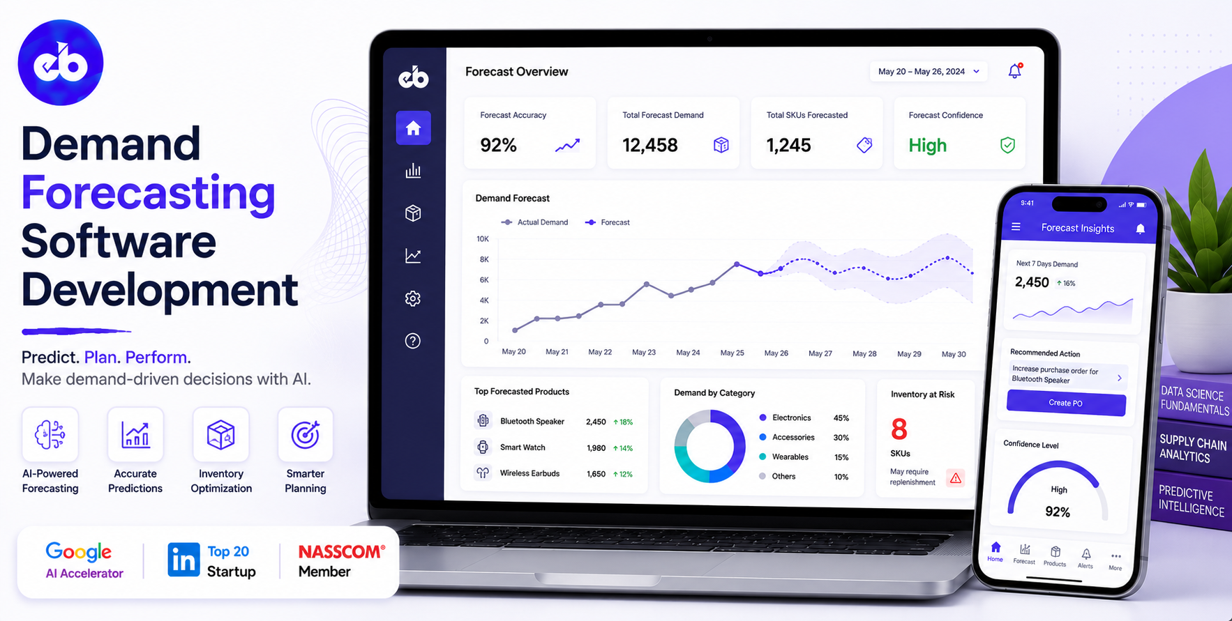
Inventory optimization is the most financially impactful problem in supply chain management. A company that holds too much inventory bleeds working capital, every rupee tied up in excess stock is a rupee not invested in growth.
A company that holds too little loses sales, every stockout is revenue that goes to a competitor and a customer whose trust degrades. The optimal inventory position is the one that satisfies demand with the minimum possible stock, and the only way to achieve it is to forecast demand accurately.
Most companies forecast with spreadsheets and hindsight. A spreadsheet that averages last month’s sales and adds 10% for growth is not a demand forecast, it is a guess with extra steps.
A genuine demand forecasting platform uses machine learning to identify the patterns that drive demand, seasonality, price elasticity, promotional lift, weather effects, macroeconomic signals, and produces forecasts by SKU, by location, by week that are measurably more accurate than any spreadsheet approach.
EngineerBabu built supply chain intelligence for Simba Beer, optimising inventory across a multi-geography distribution network, and enterprise operations for Adani Group. Google AI Accelerator 2024 Top 20. CMMI Level 5. Contact: mayank@engineerbabu.com
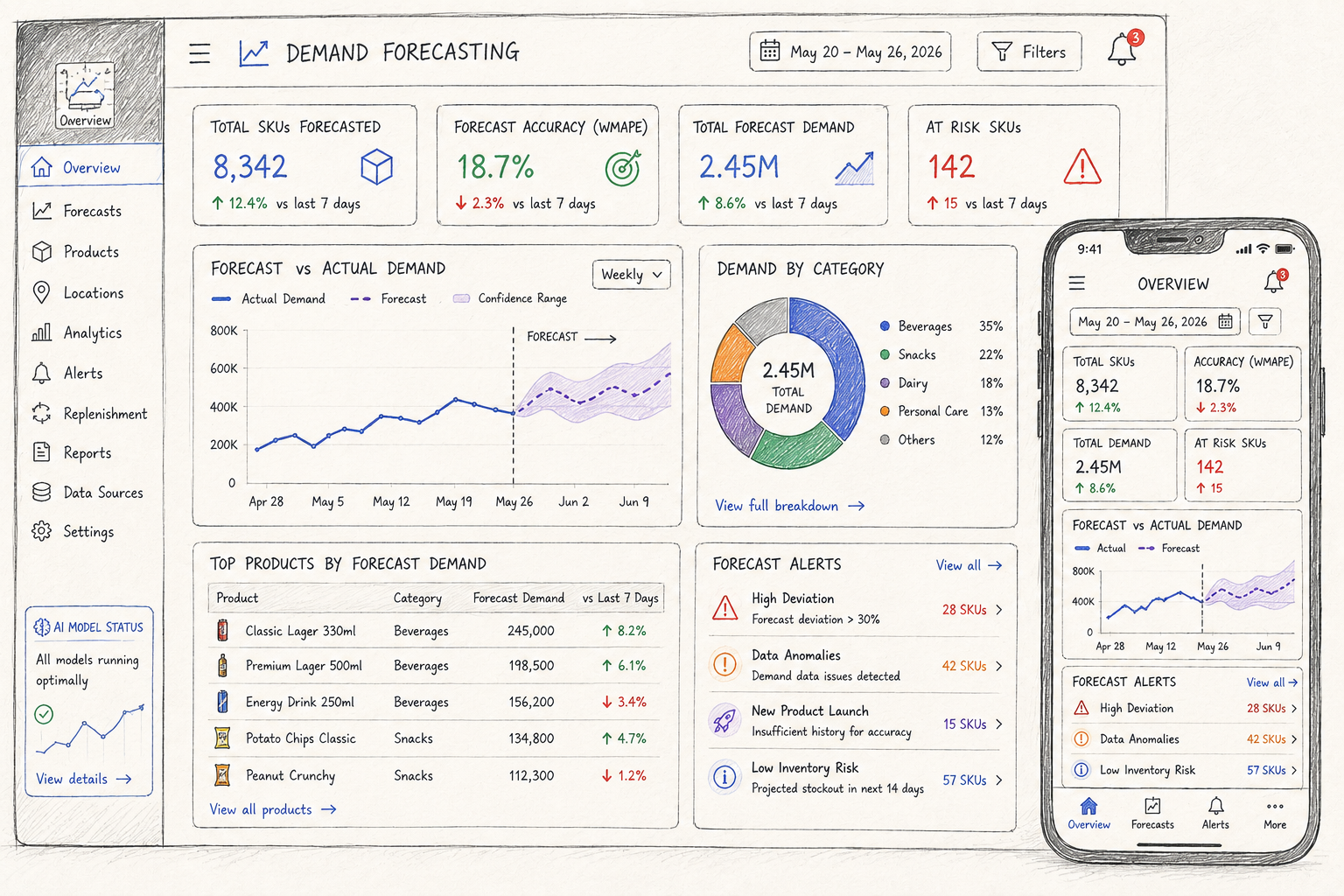
| Function | Module |
| Demand signal ingestion | Sales data, POS data, order data from all channels |
| Feature engineering | Identifying the signals that drive demand |
| Statistical baseline forecasting | Classical time-series models |
| ML demand forecasting | Gradient boosting, neural networks, ensemble models |
| External signal integration | Weather, events, economic indicators, promotions |
| New product forecasting | Analogous product approach for launches |
| Forecast accuracy measurement | MAPE, WMAPE, bias tracking |
| Safety stock calculation | Optimal buffer stock per SKU per location |
| Replenishment recommendations | Suggested orders per SKU per location |
| Exception management | Large forecast deviations surfaced for review |
| Consensus planning | Sales + supply chain alignment on final forecast |
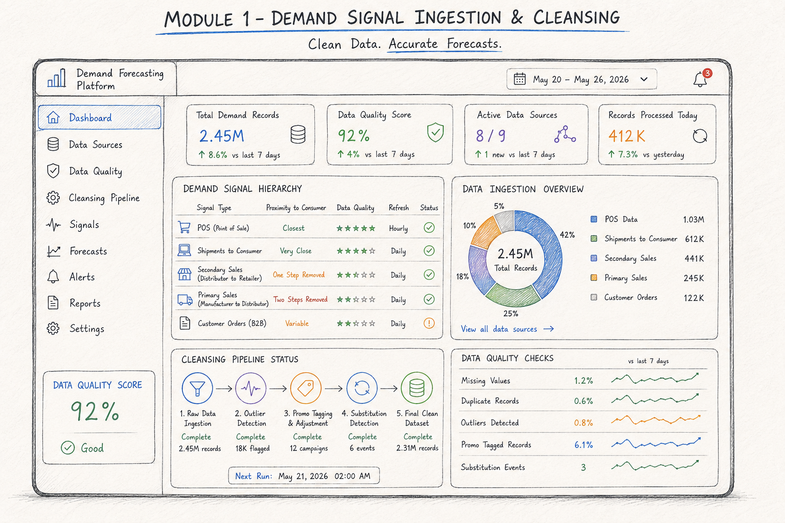
Demand forecasting is only as good as the demand data feeding it. A platform that forecasts from distributor orders is forecasting demand once removed from actual consumer demand, and distributor ordering patterns include noise (forward buying before a price increase, order batching effects) that obscures the true underlying signal.
Demand signal hierarchy, closest to consumer demand is best:
| Signal Type | Proximity to Consumer | Data Quality | Collection Complexity |
| POS (point of sale) scanner data | Closest, actual consumer purchases | Highest | High, retail partnerships required |
| Shipments to consumer (e-commerce) | Very close | High | Medium |
| Secondary sales (distributor to retailer) | One step removed | Medium | Medium |
| Primary sales (manufacturer to distributor) | Two steps removed | Medium | Low |
| Customer orders (B2B) | Depends on customer type | Variable | Low |
The demand data cleansing pipeline:
Raw demand data is never clean enough to forecast from directly. The cleansing pipeline handles:
Classical statistical models are fast, interpretable, and effective for demand patterns with clear structure. They form the baseline layer of a production demand forecasting system.
Model selection by demand pattern:
| Model | Best For | Key Characteristics |
| Moving Average | No trend, no seasonality | Smooths noise, assumes future = weighted past |
| Exponential Smoothing (ETS) | Trend + seasonality | Adaptive weighting, recent data weighted more |
| Holt-Winters | Strong seasonality + trend | Separate trend and seasonal components |
| ARIMA | Autocorrelated demand patterns | Captures lag relationships in demand |
| SARIMA | Seasonal ARIMA | ARIMA with explicit seasonal component |
| Croston’s method | Intermittent demand | Separately models demand interval and demand size |
| Prophet (Facebook) | Holiday effects + multiple seasonalities | Handles irregular calendar effects |
The model selection engine:
Rather than applying one model to all SKUs, the platform runs multiple models per SKU during the historical period, measures accuracy using cross-validation, and selects the model with the lowest error for production forecasting. This automated model selection, over thousands of SKUs, is what makes a forecasting platform more valuable than a forecasting spreadsheet.
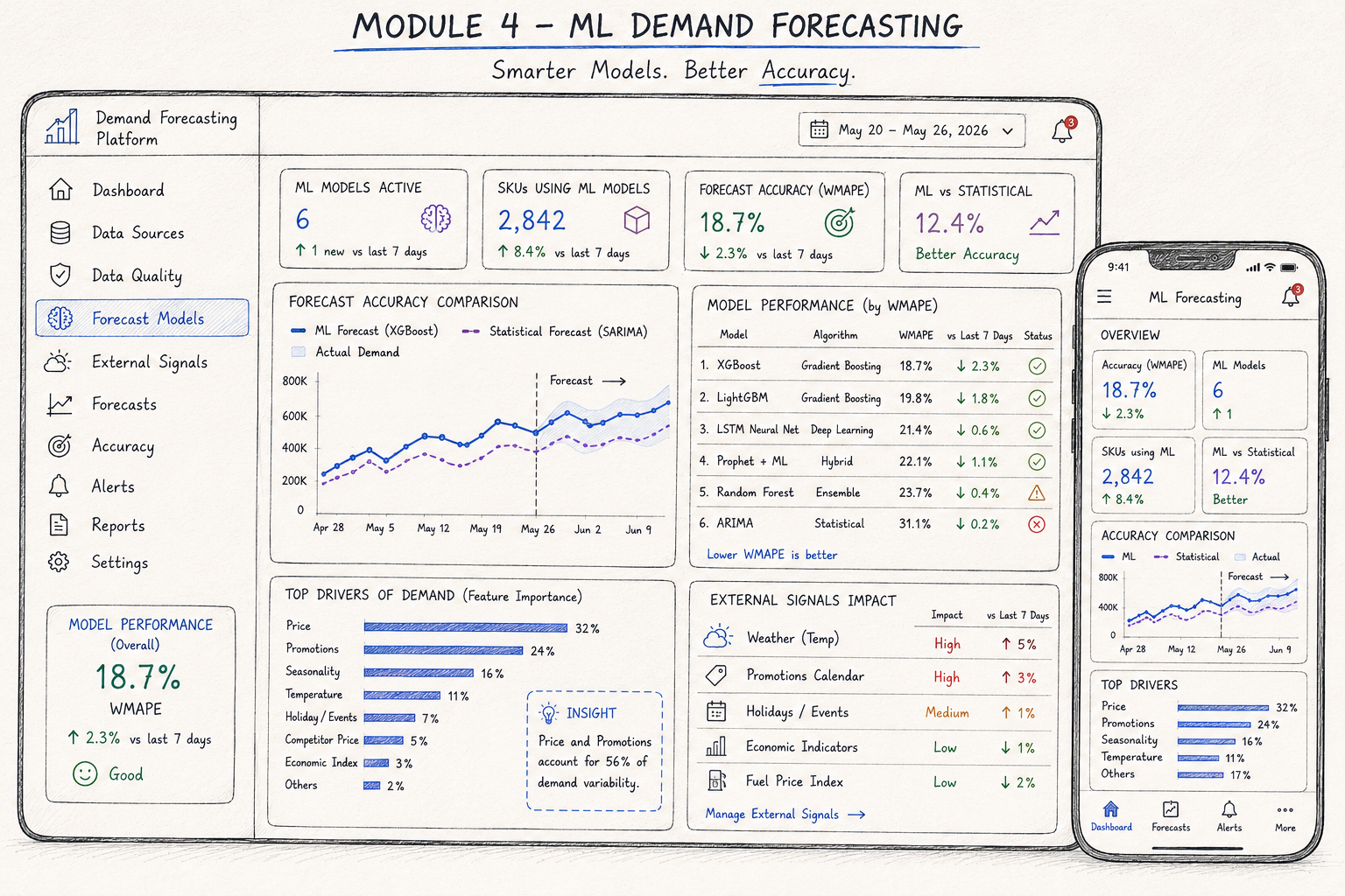
ML models capture patterns that classical models miss, particularly the impact of external variables (weather, promotions, economic indicators, competitor actions) on demand. For high-value SKUs and complex demand patterns, ML models consistently outperform classical methods.
Feature engineering, the variables that drive demand:
| Feature Category | Specific Features | How Generated |
| Calendar | Day of week, week of month, month, quarter, holidays | Calendar library |
| Seasonality | Week of year, holiday proximity | Calendar + product history |
| Price | Current price, price vs average, price change flag | Pricing system integration |
| Promotions | Is promotion active? Discount depth? Channel? | Promotion calendar |
| Weather | Temperature, rainfall, humidity, for relevant categories | Weather API |
| Distribution | Number of active outlets, new outlet openings | Distribution data |
| Macroeconomic | CPI, consumer confidence, fuel prices | Economic data feeds |
| Lag features | Sales 1 week ago, 4 weeks ago, 52 weeks ago | Historical sales |
| Rolling averages | 4-week MA, 13-week MA, 52-week MA | Computed features |
| Competitor signals | Competitor price changes, stock-outs (where available) | Market intelligence |
ML models used:
| Model | Why Used | Best For |
| LightGBM / XGBoost | Fast, handles tabular data well, interpretable feature importance | Most SKU categories |
| LSTM (Long Short-Term Memory) | Captures long-term temporal dependencies | Complex seasonal patterns |
| Temporal Fusion Transformer | State-of-the-art for multi-horizon forecasting | Premium accuracy requirements |
| DeepAR (Amazon) | Probabilistic forecasting, returns confidence intervals | Uncertainty quantification |
| Ensemble | Weighted combination of multiple models | Maximum accuracy |
Probabilistic forecasting:
Rather than a single point forecast (“you will sell 842 units next month”), a probabilistic model returns a distribution of likely outcomes, the P10, P50, and P90 forecast. The P50 is the median forecast.
The P10 means “there is a 10% chance demand will be below this number.” The P90 means “there is a 90% chance demand will be below this number.” This distribution is what drives safety stock calculations, a risk-averse inventory policy uses the P80 or P90 as the target, a lean policy uses the P50.
Classical time-series and ML models require historical data. A new product has none. New product forecasting uses analogous product methods, identifying existing products whose demand patterns most closely resemble what the new product is expected to exhibit.
The analogous product approach:
The launch curve model:
New products typically follow an S-curve adoption pattern, slow initial uptake, acceleration as awareness builds, plateau at steady-state. The platform fits a launch curve model based on the new product’s category norms and adjusts based on the planned promotional investment.
Safety stock is the buffer inventory held to protect against demand uncertainty and supply variability. Too much safety stock wastes working capital. Too little creates stockouts.
The safety stock formula:
Safety Stock = Z × σ(demand) × √(Lead Time)
Where:
Z = service level factor (Z = 1.65 for 95% service level)
σ(demand) = standard deviation of demand during lead time
Lead Time = supplier replenishment lead time in the same units as demand
Safety stock by product tier:
| Product Tier | Service Level Target | Safety Stock Approach |
| A items (top 20% by value) | 99%+ | Higher Z score, tighter safety stock, more frequent review |
| B items (next 30%) | 95% | Standard safety stock calculation |
| C items (bottom 50% by volume) | 90% | Lean safety stock, accept higher stockout risk |
| Seasonal items | 98% at peak | Elevated pre-season stock build |
| Promotional items | 99% | Additional buffer for promotional launch |
Dynamic safety stock:
Rather than a fixed safety stock calculated annually, the platform recalculates safety stock weekly based on the current demand volatility (which changes with season, promotions, and market conditions) and the current supplier lead time (which changes with supplier capacity, port congestion, and logistics conditions).
A supplier whose lead time increased from 14 to 21 days needs a proportionally higher safety stock, the platform adjusts automatically.
Automated replenishment recommendations:
The forecasting platform produces a weekly replenishment recommendation per SKU per location, how much to order, from which supplier, by when, to arrive when needed.
| Output | Details |
| Recommended order quantity | Based on forecast + safety stock − projected inventory at reorder point |
| Order timing | When to place the order (today, in 3 days, in 1 week) |
| Suggested supplier | Primary supplier or backup based on current lead times |
| Urgency level | Standard / Priority / Urgent based on days of stock remaining |
| Auto-approve flag | Low-risk, routine orders can be auto-approved; unusual orders go to buyer review |
Consensus forecasting:
The statistical/ML forecast is the starting point, not the final word. Sales teams know about distribution expansion plans, upcoming promotions, and customer commitments that are not yet in the historical data. Operations teams know about planned plant shutdowns or supplier lead time changes.
The consensus planning module allows sales and supply chain teams to see the statistical forecast and override it with their commercial intelligence, with a required justification for any override above a defined threshold. The final consensus forecast is what drives replenishment.
| Module | Cost Range (USD) | Notes |
| Demand signal ingestion + cleansing | $8K – $15K | Multi-source, outlier detection, promo tagging |
| Classical time-series models | $8K – $15K | ETS, SARIMA, Prophet, model selection engine |
| ML forecasting models (LightGBM + LSTM) | $12K – $22K | Feature engineering + model training pipeline |
| External signal integration (weather, promo, macro) | $6K – $12K | API integrations |
| New product forecasting (analogous method) | $5K – $10K | |
| Probabilistic forecasting output | $5K – $10K | P10/P50/P90 distribution |
| Safety stock optimisation engine | $6K – $12K | Dynamic, tiered calculation |
| Replenishment recommendation engine | $6K – $12K | Auto-approve logic |
| Consensus planning workflow | $5K – $10K | Override capture, justification |
| Forecast accuracy tracking (MAPE, WMAPE, bias) | $5K – $10K | |
| Analytics dashboard | $5K – $10K | |
| AWS + VAPT + Year 1 ops | $5K – $10K | |
| Total | $76K – $148K | Full demand forecasting platform |
EngineerBabu built supply chain intelligence for Simba Beer and enterprise operations for Adani Group. Google AI Accelerator 2024 Top 20. CMMI Level 5. Contact: mayank@engineerbabu.com
MAPE (Mean Absolute Percentage Error) is the most widely used metric for measuring demand forecast accuracy. It calculates the average absolute percentage difference between the forecast and actual demand: MAPE = (1/n) × Σ(|Actual − Forecast| / Actual) × 100. A MAPE of 15% means the forecast was wrong by an average of 15% across the measured periods. MAPE has one important limitation, it is undefined when actual demand is zero, making it inappropriate for intermittent demand SKUs. For those, WMAPE (Weighted MAPE, weights errors by actual demand volume) or MAE (Mean Absolute Error) is preferred. In practice, supply chain teams track forecast bias (whether the forecast systematically over- or under-predicts) alongside MAPE, a low-MAPE forecast with systematic bias still produces stockouts or excess stock in predictable patterns.
Demand forecasting uses historical data and statistical models to predict demand weeks to months into the future, producing a medium-term plan that drives replenishment, production scheduling, and capacity planning decisions. Demand sensing uses short-term signals, typically point-of-sale data, order patterns, and search trends from the past 1 to 7 days, to create a very short-term forecast for the next 1 to 2 weeks, improving on the medium-term forecast as the time horizon shortens. Demand sensing is most valuable for FMCG companies with daily replenishment cycles, where a 10 to 15% improvement in 1-week forecast accuracy translates directly into reduced safety stock requirements. A comprehensive demand platform implements both: medium-term ML forecasting for planning and procurement, and demand sensing for short-term execution and distribution optimisation.
Seasonal demand, beer sales that peak in summer, air conditioner sales that spike before monsoon, gift hamper sales that surge before Diwali, requires models that explicitly capture seasonal patterns rather than treating them as noise. The platform uses SARIMA (Seasonal ARIMA) and ETS models with seasonal components for products with annual seasonality, and augments these with calendar features (week of year, distance from major holidays, temperature, particularly relevant for beverages) in the ML models. For products with strong seasonality, the platform also generates pre-season stock build recommendations, identifying the point at which the company must begin building inventory to satisfy peak demand without creating excess stock in the off-season. The Simba Beer engagement at EngineerBabu involved exactly this challenge, optimising pre-season builds and distribution deployment across a multi-geography network.